 Damodaran (2011) explained that there were three methods by which to calculate a prospective Equity Risk Premium. The first is to survey investors and academics, in a similar fashion to Welch (2000). The second is to base the calculation on historical equity returns against an appropriate risk-free rate and the third is to use “market rates or prices on traded assets today”. (Damodaran 2011, p.15). It is a variation on this last method that we will adopt. In an earlier article we looked at a method employed by Dimson et al (2002) to calculate the Equity Risk Premium (ERP). We will now develop this with the data available to us, which allows the calculation of the ERP between 1976 and 2012, and the volatility index (VIX) levels from 1989 to 2012. I propose to look at three time periods, 1980 to 1989, 1980 to 1999 and 1980 to 2009 and calculate the ERP as discussed earlier, by taking Risk into account. This will enable us to use an adjusted historical arithmetic mean premium which may be used as a prospective premium. By using the aforementioned time periods, we can then check this forecast against the actual which will permit us to make a judgement on the validity of the assumptions. Performing this over a greater timeframe would be beneficial but as we are constrained by the data, it is reasonable to experiment with this and see if it warrants deeper investigation. To support this approach, Damodaran (2011, p.45) said that “option prices can be used to back out implied volatility in the equity market. To the extent that the equity risk premium is our way of pricing in the risk of future stock price volatility, there should be a relationship between the two. The simplest measure of volatility from the options market is the VIX.”
It is worth remembering at this point that we will not detail the statistical assumptions that allow us to make this calculation as they are out with the scope of this article. To provide a level of comfort though, Gregory (2007 p.4) also uses this rationale by saying if “expected returns are lognormally distributed, from Jensen’s inequality, the arithmetic average risk premium should be approximately the geometric average risk premium plus half the variance”. As discussed earlier, we may calculate a different percentage of the variance so we will also use half as a comparison. We read in a previous article that indices around the world are closely correlated, allowing us another assumption, that the VIX is a reliable indicator of Risk for the FTSE All Share. I propose to look at each of the periods and use the VIX valuation for the month immediately afterwards, thereby allowing an estimate of a prospective Equity Risk Premium. In addition, I will also use the 0.5 multiple, as described earlier. This will give us two figures to compare against actual. Figure 1 below shows the descriptive statistics for the ERP, 1980 to 1989, using our data from the FTSE All Share and All Government Bonds. Click on images to enlarge.
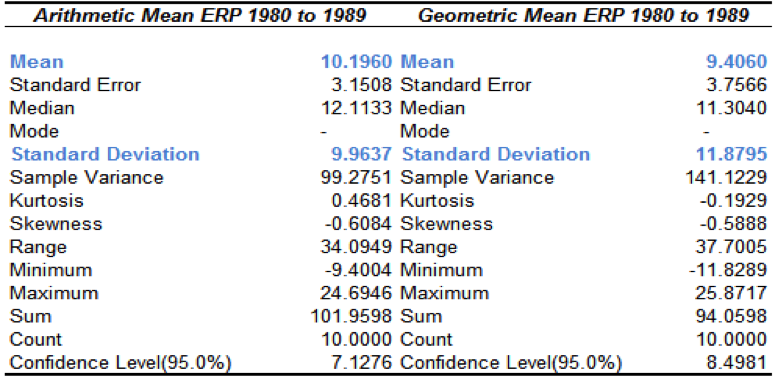
Figure 1: Equity Risk Premium (ERP) Means 1980 to 1989
As a reminder of the formula:
Factor of the variance (multiple) = Δ between arithmetic and geometric means / standard deviation2
Δ between arithmetic and geometric means = 10.1960 – 9.4060, this give us 0.79
9.96372 (standard deviation squared)= 99.2753
We can then solve for the multiple as follows:
multiple = (0.79/.99.2753) x 100
multiple = 0.7958
The arithmetic mean will exceed the geometric mean by this factor in the variance in annual returns. This figure, 0.7958, we will now use as the multiple on the VIX value to calculate a prospective arithmetic mean.
Dimson et al (2002 p.184), recalculated the historical ERP by adjusting it by “projections of early twenty-first century volatility”. For our example, we must return to the twentieth century. On the 31st of January 1990, the VIX stood at 25.36. We must use this figure as our data starts at this point for the index. Making the same assumptions as earlier, we multiply:
0.7958 by 0.25362, which gives us 0.0512, or 5.12%.
This is the amount by which the arithmetic mean will exceed the geometric mean. We have established that for this period the geometric mean was 9.4060, as can be seen in Figure 27, therefore a reasonable assumption for a forward looking Equity Risk Premium would be 9.4060 plus 5.12%, which is 14.526. At this point we must include the standard error, which in this instance is 3.1508. This gives us a range for the prospective Equity Risk Premium of 11.3752 to 17.6788. In Dimson et al’s (2002) example, the standard error was approximately one–tenth. With our data it is closer to one-third (3.1508/9.9637). The standard error also tells us that there is roughly a two-thirds chance that the prospective ERP will fall into this range. Calculating the arithmetic mean premium for 1990 to 2009 we have 0.7621, from 1990 to 1999 it is 4.1416. This is respectively five and three standard errors from the mean.
If we use 0.5, as propounded by Dimson et al (2002), we would have the following:
0.5 x 0.25262 =0.0322, or 3.2156%.
This would have given us a range, at one standard error, of 6.1904 to 12.5568. Effectively, neither of our calculations would have been of much use, although the latter version is closer to the actual ERP. From 1990 onwards there were turbulent times in indices across the globe, these macro factors impacted the FTSE All Share and the total equity returns. We will consider these after looking at two further examples of attempting to calculate a prospective ERP.
Having looked at a ten year period, we will now extend this to twenty and discover if it presents a more accurate estimation of a prospective ERP.
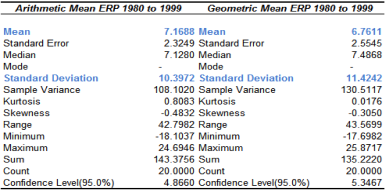
Figure 2: Equity Risk Premium (ERP) Means 1980 to 1999
As in the previous example, we will follow the steps in the calculation:
Factor of the variance (multiple) = Δ between arithmetic and geometric means / standard deviation2
Δ between arithmetic and geometric means = 7.1688 – 6.7611, this give us 0.4077
10.39722 (standard deviation squared)= 108.1018
We can then solve for the multiple as follows:
multiple = (0.4077/108.1018) x 100
multiple = 0.3771
On the 31st of January 2000, the average value for the VIX over the last ten years stood at 18.6114. We can again calculate the amount by which the arithmetic should exceed the geometric mean, given a current risk level:
0.3771 x 0.18612 = 0.0131, or 1.306%.
The geometric mean was 6.7611, plus 1.306 is 8.0671. This is our revised forward looking Equity Risk Premium, based on twenty years of returns. In this instance, the standard error is 2.3249, giving us a range of 5.7422 to 10.392. In the previous example, the actual Equity Risk Premium for 1990 to 2009 was 0.7621. As with ten years of data, actual figure is four standard errors from our prediction. If we look at 2000 to 2009, the actual ERP was -2.1675, five standard errors from our prediction. As with the previous data set, we will also compare by using the 0.5 multiple:
0.5 x 0.18612 = 0.0173, or 1.7317%
This would have given us a prospective ERP of 8.4928%. Once again it is four and five standard errors from the actual values. We have a final data set to look at before we can consider some of the reasons why our predictions are not accurate. In the next example we will look at the data from 1980 to 2009, a thirty year period.
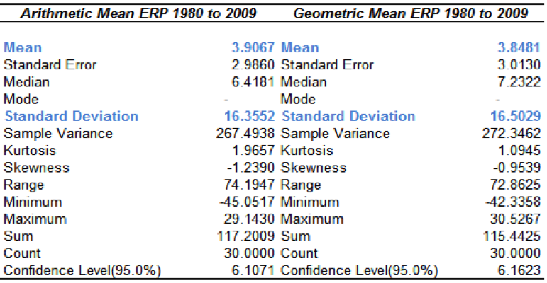
Figure 3: Equity Risk Premium (ERP) Means 1980 to 2009 (Appendix 5)
We now follow the same steps as before:
Factor of the variance (multiple) = Δ between arithmetic and geometric means / standard deviation2
Δ between arithmetic and geometric means = 3.9067 – 3.8481,this give us 0.0586
16.35522 (standard deviation squared)= 267.4926
We can then solve for the multiple as follows:
multiple = (0.0586/267.4926) x 100
multiple = 0.0219
On the 29th of January 2010 the VIX average for the past twenty years stood at 20.2452. Therefore the prospective value may be calculated as follows:
0.0219 x 0.20252 = 0.0009, or 0.089%.
The geometric mean was 3.8481; therefore our forecast for a prospective arithmetic mean ERP is 3.9371. Within one standard error (2.9860), the range is 0.9511 to 6.9321
Looking again at the remainder of our data, 2010 and 2011, the arithmetic mean ERP is -4.7790. In common with the previous examples, we are three standard errors away from our forecast. If we used 0.5 as the multiple, we would have had:
0.5 x 0.20252 = 0.0205, or 2.0503%.
This would have given a prospective Equity Risk Premium of 5.8984%. We are looking at a short timescale of only thirty years, and in this last example comparing to only two years, but it does provide some insight into how difficult it is to gauge a prospective ERP using a current risk value. It is true that the last thirty years have seen some tremendous market upheaval and it is worth considering some of the behavioural aspects of this period to see if that can help explain why it is so difficult to calculate a future ERP. In a future article, and in order to put these results into context, we will also compare them to the thinking on the historical Equity Risk Premium and draw conclusions on the values discussed by some of the academics we have already mentioned. Still on the theme of a prospective ERP, dividends are another method by which one may calculate a prospective ERP, and we will look at that next time.
References
- Damodaran, A. (2011) Equity Risk Premiums (ERP): Determinants, Estimation and Implications – The 2011 Edition Stern School of Business
- Dimson, E., Marsh, P., and Staunton, M. (2002) Triumph of the Optimists: 101 Years of Global Investment Returns Princeton University Press
- Gregory, A. How Low is the UK Equity Risk Premium? XFi Centre for Finance and Investment, University of Exeter (2007)
- Welch, I. Views of Financial Economists on the Equity Premium and on Professional Controversies Journal of Business Vol 73 No 4 2000
Twitter: @MillarAllan @seeitmarket
Any opinions expressed herein are solely those of the author and do not in any way represent the views or opinions of any other person or entity.

: Showing Some Signs of Emerging Strength")
