Since this is my first post on See It Market, I thought I’d offer up a little bit of background on our model and method of analysis. First and foremost, the following is not created with predictive near-term price action in mind. It gets at the heart of current stock market valuations based on a number of inputs over history.
At Global Technical Analysis, we believe that the chief determinant of future total returns is the relative valuation of the stock market index at the time of purchase (in this case, the S&P 500 Index).
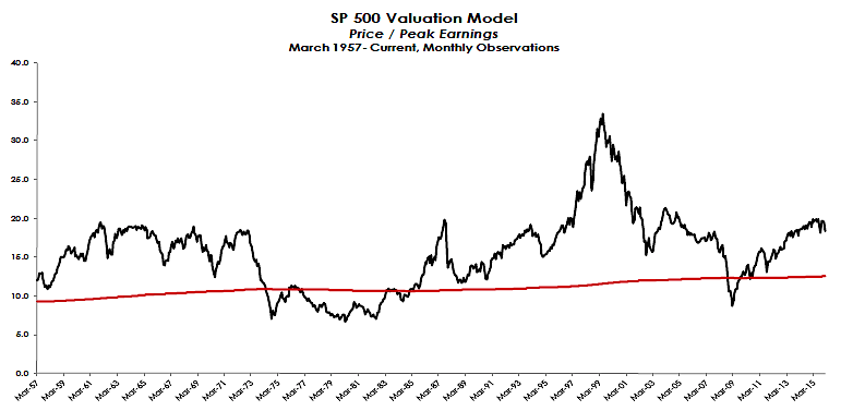
We measure stock market valuation using the Price/Peak Earnings multiple as advocated by Dr. John Hussman. We believe the main benefit of using peak earnings is the inherent conservatism it affords: it is not subject to analyst estimates, not subject to the short-term ebbs and flows of business, and not subject to short-term accounting distortions. Annualized total returns can be calculated over a horizon period for given scenarios of multiple expansion or contraction.
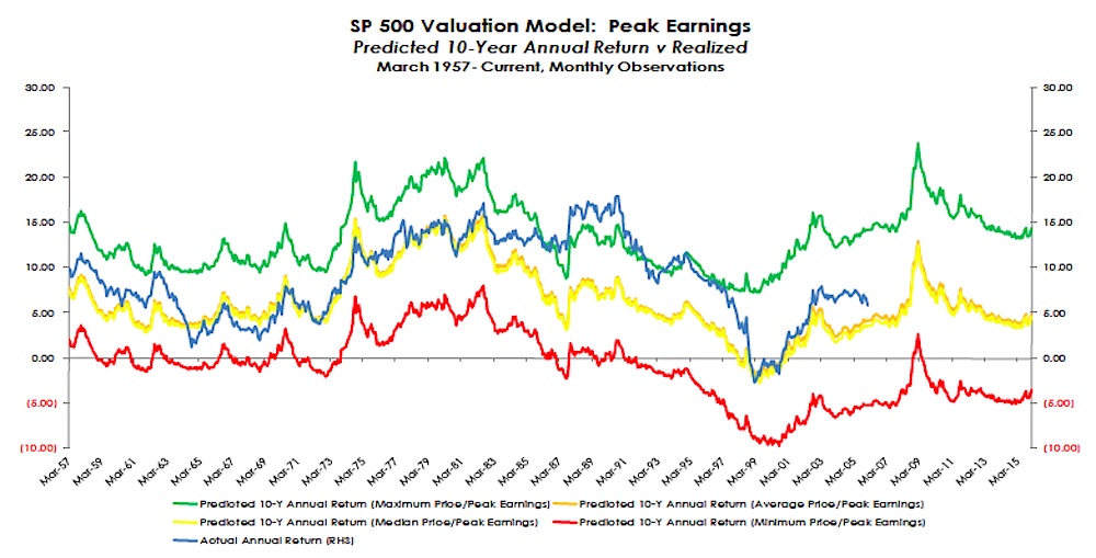
Our analysis highlights expansion/contraction to the minimum, mean, average, and maximum multiples (our data-set begins in January 1900) . The baseline assumptions for growth and horizon period are 6% and 10 years, respectively. We also provide graphical analysis of how predicted returns compare to actual returns historically.
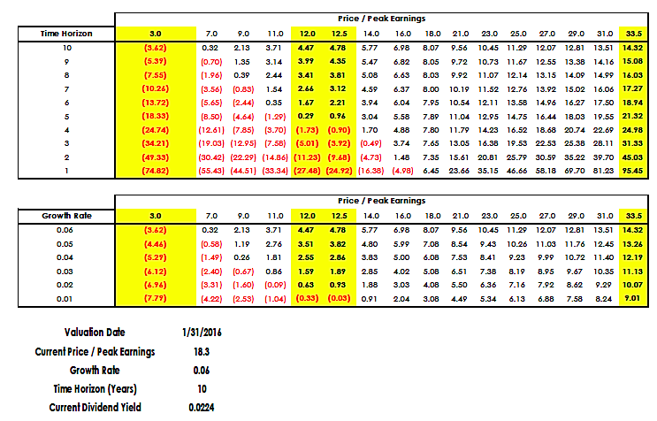
We provide sensitivity analysis to our baseline assumptions. Amongst the images below, you’ll find a couple of sensitivity tables. The first sensitivity table, ceterus paribus, shows how future returns are impacted by changing the horizon period. The second sensitivity table, ceterus paribus, shows how future returns are impacted by changing the growth assumption.
We also include the following information in our analysis: duration, over(under)-valuation, inflation adjusted price/10-year real earnings, dividend yield, option-implied volatility, skew, realized volatility, historical relationships between inflation and p/e multiples, and historical relationship between p/e multiples and realized returns.
Once again, our analysis is not intended to forecast the short-term direction of the S&P 500 Index. The purpose of our analysis is to identify the relative stock market valuation and inherent risk offered by the index currently.
Predicted Returns
Predicted Returns – Sensitivity Analysis
Price To Peak Earnings
To get at the significance of the P/E, you have to start by understanding that stocks are not a claim to earnings anyway. Stocks are a claim to a future stream of free cash flows – the cash that can actually be delivered to shareholders over time after all other obligations have been satisfied, including the provision for future growth. Knowing this already tells us a lot. For example, price/earnings ratios based on operating earnings are inherently misleading, since that “earnings” figure does not deduct interest owed to bondholders nor taxes owed to the government. This isn’t to say that P/E ratios are useless, but it’s important for the “E” chosen by an investor to have a reasonably stable relationship to what matters, which is the long-term stream of free cash flows . For that reason, our favored earnings measure for stock market valuation (though it can’t be used for individual stocks) is “peak earnings” – the highest level of net earnings achieved to date. (This is excerpted from Dr. John Hussman)
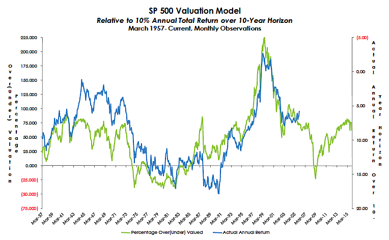
Valuation
As of 01/31/2016: Overvalued by 62.5%.
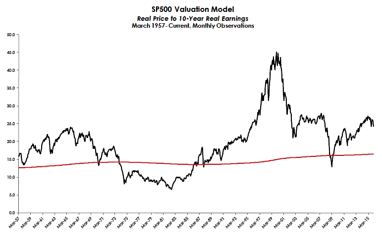
Inflation Adjust P/E
As of 01/31/2016: Real Price to 10-Year Real Earnings 24.3x
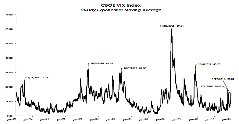
CBOE VIX Index 10 Day Exponential Moving Average
VIX measures 30-day expected volatility of the S&P 500 Index. The components of VIX are near- and next term put and call options, usually in the first and second SPX contract months. “Near-term” options must have at least one week to expiration; a requirement intended to minimize pricing anomalies that might occur close to expiration. As of 01/31/2016: 10-Day EMA 23.02
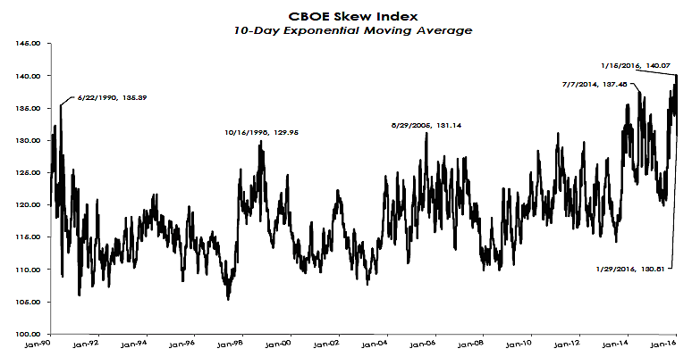
CBOE SKEW Index 10 Day Exponential Moving Average
The CBOE SKEW Index (“SKEW”) is an index derived from the price of S&P 500 tail risk. The price of S&P 500 tail risk is calculated from the prices of S&P 500 out-of-the-money options. SKEW typically ranges from 100 to 150. A SKEW value of 100 means that the perceived distribution of S&P 500 log-returns is normal, and the probability of outlier returns is therefore negligible. As SKEW rises above 100, the left tail of the S&P 500 distribution acquires more weight, and the probabilities of outlier returns become more significant. As of 01/31/2016: 10-Day EMA 130.81
Thanks for reading.
Twitter: @Techs_Global
The author may hold S&P 500 related securities at the time of publication. Any opinions expressed herein are solely those of the author, and do not in any way represent the views or opinions of any other person or entity.
 Rolling Over At Key Fibonacci Level?")


