 By Allan Millar
In my last article we considered historical risk premiums and explored means for quantifying Equity Risk Premium. Taking that one step further, we shall now turn our attention to calculating a prospective value of Equity Risk Premium (ERP).
There is obviously no way to predict the future so the most common way to predict the Equity Risk Premium is to determine what it has been in the past. As we have seen, this is not an easy task and can provide different answers, even within the same time period and data set. Dimson et al (2002 p.188) also highlight the fact that “Financial economists may be reluctant to diverge markedly from the historical mean.” They also point out a number of factors which need to be taken into account – relying on historical computations of the ERP, acknowledging that expectations for the risk premium may change and that stock market indices are affected by many factors.
In an earlier article we noted the comments by Ilmanen (2011) and Cochrane (2011) with respect to calculating a prospective Equity Risk Premium. Given these arguments, how should it then be calculated so that we may confidently predict the value? Dimson et al (2002) suggest that when making decisions about the future we should use the arithmetic mean, rather than the geometric mean because we must remember that if we look at total returns on an annual basis, there will be considerably more volatility than when we examine the returns over a longer time period. As we have read, using the arithmetic mean allows the calculation of the return expected in any given year and it is then also possible to calculate standard deviations which will give us the fluctuations around the mean. I propose to do this for the UK data available and will analyse in a future article. In order to demonstrate this I’ll look at the ERP for the period 1980 to 2009, data which we will use more fully later.
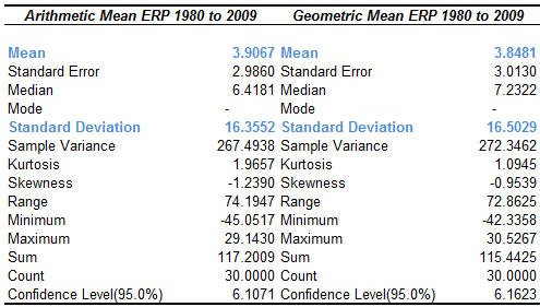
Figure 1: FTAS Arithmetic and Geometric Mean ERPs (Source Thomson Datastream)
It is evident from Figure 1 that the Equity Risk Premium is volatile. For this time period there is a mean of 3.9067 and 3.8481 for arithmetic and geometric respectively, with standard deviations of 16.3552 and 16.5029. From this data we can calculate the amount by which the arithmetic mean will exceed the geometric mean by a factor of the variance in annual returns. This was done by Dimson et al (2002) who calculated this difference for sixteen nations and found it approximately equal to one-half of the variance of the annual returns. The statistical assumption they use is that the arithmetic and geometric means will be linked by the standard deviation of returns if the returns are lognormally distributed. From the formula below, we can work back to look at the multiple for our data and we shall briefly look at the methodology after an example using our ERP figures for UK equities and gilts. Their study was based on 101 years of data; we are constrained by the data at our disposal. Given the information in Figure 1 above, we can arrive at our own value. First to confirm the formula we will use:
Factor of the variance (multiple) = Δ between arithmetic and geometric means / standard deviation2
Δ between arithmetic and geometric means = 3.9067 – 3.8481, this give us 0.0586
16.35522 (standard deviation squared)= 267.4926
We can then solve for the multiple as follows:
multiple = (0.0586/267.4926) x 100
multiple = 0.0219
We can then say that we would expect the arithmetic mean to be greater than the geometric mean by 0.0219 times the variance of the annual returns. This is considerably less than the 0.5 used by Dimson et al (2002) and at first reading this looks unlikely but in a future article, when we look in detail at the FTSE All Share over the last 36 years, we will see if it is a useful predictor for a prospective Equity Risk Premium. From our data we also know that the standard error is 2.9860. Looking at the period from 1980 to 2009, we know that the arithmetic mean is 3.9067. We can therefore only be 66.67% certain that the true mean lies within one standard error of this number, giving us a range of 0.9207 to 6.8927. This wide fluctuation in the value is an explanation of why it is best to look at returns over the longest possible time period. As we can see in Figure 1 above, arithmetic means are volatile but in our example are not much higher than the geometric means. Dimson et al (2002 p.182), explain this by saying that for “stable assets the arithmetic mean risk premium is only slightly above its geometric counterpart,” a finding borne out by their extensive research. However, is it possible to calculate a prospective Equity Risk Premium, given the volatility in indices around the world? Looking at the period in question, the years in which there have been the most turmoil, be it financial, political or terrorist or natural disaster, the volatility is at its highest. Considering terrorist incidents, Glassman (2006) provided a perspective about the impact of the events of September 2001 and the impact is visible in the FTSE All Share. The total return in August 2001 was not surpassed until June 2005, the gradual increase from that point then being halted by Lehman and the Financial Crisis. The point that Glassman makes is that since 2001, there has been a discount subsequently priced into equities. If we look at the total returns in 2005, they were greater at the end of July, after the London bombings, than they were in June. As Glassman notes, it isn’t possible to definitively identify this discount but it may well be a reasonable assumption that the market (p34) is compensating for “unknown geopolitical risk.” To further illustrate this point, the FTSE All Share stood at 14,331 on August 2001, with the exception of March 2002; it would not be at this level again until November 2004. In June 2005, the index was at 16,032 and the events of July 2005 had no impact. The index, as noted continued to rise until the onset of the Financial Crisis.
Unfortunately for investors, these historical events are very unlikely to be repeated exactly and of course the timing of any such events is almost impossible to predict. Perhaps the only certainty is that there will be events which will impact upon returns. Therefore, all we can do when considering the arithmetic means of the future, is to make assumptions based on current predictions. Dimson et al (2002) addresses this by looking at factoring in recent risk. They identified a risk factor and used it as the standard deviation by which we may derive the prospective arithmetic mean ERP. In effect, the formula above continues as follows:
multiple x risk2 = amount by which arithmetic mean will exceed the geometric mean
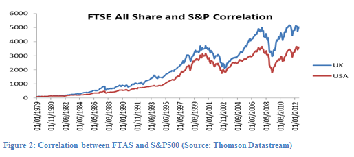
This value is then added to the historical geometric mean to provide an estimate of a future Equity Risk Premium. The issue we face is determining the risk factor. I propose to do this as well, using the CBOE VIX Model. In the absence of any other risk approximation, and being aware that the VIX index I will use refers to put and call option volatility of the S&P 500, hence exclusively looking at equities, I propose that it can be used as the standard deviation. Regarding the use of the VIX, it is obviously an approximation as it is based on US data but as we shall see, the Markets are all closely correlated. If we look at Figure 2 below, we can see that the correlation is close and over this period it is 0.7287. This data is for the period from 1979 to 2012 and is based on the FTSE All Share and the S&P 500.
As we mentioned earlier, Dimson et al (2002) arrived at multiple of approximately 0.5, saying that this estimate is accurate for lognormal distributions. In their study, when this multiple was applied to the squared standard deviation of returns, the answer was continually close to the difference between the arithmetic and geometric means. We may calculate the multiple thereby showing the difference between arithmetic and geometric means based on an up to date risk model. As we have seen, we do not match Dimson et al’s (2002) value. This may be because our returns are not lognormally distributed so in one of my next articles we will calculate using our multiple and Dimson’s. It is worth highlighting at this point that many financial models, such as Black-Scholes, assume normal changes in the logarithm but there is a case that log-Levy distributions would be more appropriate (Mandelbrot and Taleb, 2006), that is there would be a heavy tail. Considering the bell curve, it is also worth remembering Taleb’s (2010) p232 assertion that “one of the most misunderstood aspects….is its fragility and vulnerability in the estimation of tail events.” This is an intriguing topic but is out with the scope of this article. For the purposes of this exercise we will satisfy ourselves with Dimson et al’s (2002 p.182) assertion that “the approximation is very accurate if returns have a distribution that is close to lognormal.” We established earlier in that the arithmetic mean will be greater than the geometric mean by 0.0219 of the variance of annual returns. Assuming the VIX to be at 16%, essentially the volatility (the standard deviation), we have 0.0219 x 0.16², which gives us 0.056%. We can now see what the prospective Equity Risk Premium may be, with reference to the data in Figure 3:
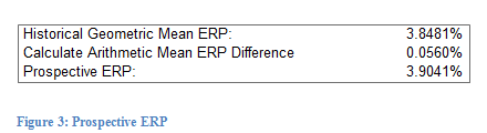
As we can see, this provides us with an expectation of the future ERP of approximately 3.9041%. In a future article we will try this for different time periods in the past and discover if it accurately predicted what did happen in the next time period.
Given what we have discussed above, should we be happy that we have an answer to predicting the future equity risk premium? Unfortunately, and we will have a more informed opinion on this later, I would suggest not. Perhaps the most significant factor is that the FTSE All Share, in common with all other markets, is susceptible to influence from many factors. As discussed, there are financial crises, natural disasters etc. Dimson et al (2002) and Damodaran (2001) propose an alternative, examining equity dividends and the possibilities they offer to calculate a prospective Equity Risk Premium. We will do that in a subsequent article, by examining the importance of reinvesting dividends and once again employing the Gordon Growth Model. By doing so we will demonstrate that the Dividend Yield may be a proxy for the risk premium.
Before making these calculations, the next article will consider the impact of behavioural finance on the Equity Risk Premium.
References
- Cochrane, J. 2011. “Discount Rates”. Presidential Address at the 2011 American Finance Association Meeting Journal of Finance, vol. 66, no. 4 (August 2011) pp1047–1108
- Damodaran, A. (2011) Equity Risk Premiums (ERP): Determinants, Estimation and Implications – The 2011 Edition Stern School of Business
- Dimson, E., Marsh, P., and Staunton, M. (2002) Triumph of the Optimists: 101 Years of Global Investment Returns Princeton University Press
- Glassman, James K. “The price of TERRORISM” Kiplinger’s Personal Finance, Vol. 60 Issue 10, October 2006 p32-34,
- Ilmanen, A. Time Variation in the Equity Risk Premium Rethinking the Equity Risk Premium (Edited by P. Brett Hammond, Jr., Martin L. Leibowitz, and Laurence B. Siegel) Research Foundation of CFA Institute (2011)
- Taleb, Nassim Nicholas (2010) The Black Swan Penguin Group 2nd Edition
- www.ft.com A focus on the exceptions that prove the rule Benoit Mandelbrot and Nassim Taleb – published March 23, 2006 16:40 | Accessed 4th August 2012
Twitter: @MillarAllan @seeitmarket
No position in any of the mentioned securities at the time of publication.
Any opinions expressed herein are solely those of the author and do not in any way represent the views or opinions of any other person or entity.


